Inspect a calibrated scalar map#
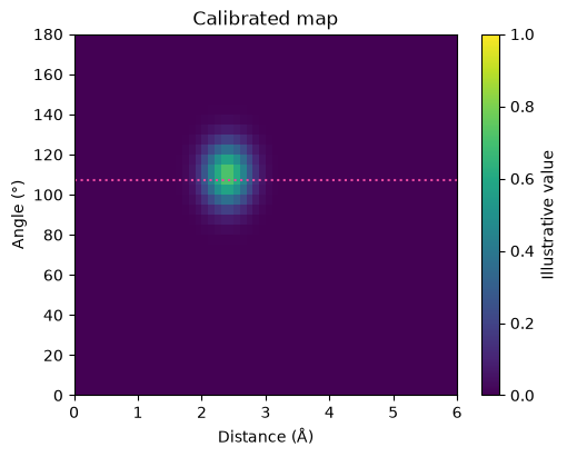
Use Plot2D when each array axis is a scientific quantity, such as distance and angle, rather than image position. This small synthetic map teaches display and selection; it is not a physical G3 calculation or a model prediction.
Run using a development build containing Plot2D. No GPU training, real-data download, or learned weights are required.
import numpy as np
import ipywidgets as widgets
import quantem.widget as qw

qw.profile(check_updates=False)
quantem.widget  0.0.1rc30
  install       editable checkout
quantem.gpu     0.0.1rc6
  install       published package
quantem         0.1.9
torch           2.14.0+cu130  device=cpu
python          3.12.14
Make a known map#
Columns are radius bin centers in Å; rows are angle bin centers in degrees. Row zero is shown at the bottom. The illustrative peak is near 2.4 Å and 110°. The 36 × 60 float64 map occupies about 17 kB before widget metadata.
Inspect with physical axes#
Hover near the peak and read its bin, radius, angle and value. Wheel to zoom, drag to pan, and select Reset View. Changing Color changes only the display. The source and hover values remain float64; browser colormapping uses float32 display buffers.
plot = qw.Plot2D(
    values, x=radius, y=angle,
    x_label="Distance (Å)", y_label="Angle (°)",
    colorbar_label="Illustrative value", title="Calibrated map",
    width=500, max_width=600, vmin=0, vmax=1, save_state=True,
)
plot
Move a reading line#
The slider selects an angle row; it does not change the data. The link is browser-local and does not require Python callbacks during dragging.
angle_slider = widgets.FloatSlider(
    value=107.5, min=2.5, max=177.5, step=5.0,
    description="Angle (°)", continuous_update=True,
)
plot.horizontal_line = angle_slider.value
angle_link = widgets.jslink((angle_slider, "value"), (plot, "horizontal_line"))
angle_slider
Replace values, keep the view#
Zoom first, then run the next cell. The same plot updates in place, retaining the grid, color limits and viewport. A second Plot2D display is not created.
plot.set_data(values * 0.75)
Obtain an editable figure#
The figure retains the current data, labels and viewport. This is a deliberate static export preview, separate from the interactive plot; it is displayed once. To save it, call figure.savefig("scalar-map.svg").
The widget follows the notebook light/dark theme. By default, saved snapshots omit the array and keep a static PNG preview. This small tutorial explicitly uses save_state=True so its complete float64 map remains interactive in supporting notebook and documentation frontends. Retain scientific data separately. Standalone HTML export is not part of this API.
figure = plot.figure()
figure