Direct ptychography

Direct methods reconstruct the phase in a single pass, with no iteration and no initial guess. They assume a weak phase object, which makes the relationship between the recorded intensities and the specimen phase linear and therefore invertible by a filter.

Run these first on any dataset. They take seconds, they tell you whether the data is usable, and they produce the aberration and rotation estimates that an iterative reconstruction needs.

Where the phase information comes from¶

When the probe is convergent, the bright-field disk you see on the detector is the unscattered beam. Any spatial frequency in the specimen scatters a second, shifted copy of that disk. Where the two disks overlap, scattered and unscattered electrons land on the same detector pixels and interfere, and it is that interference which encodes the specimen phase.

The size of the shift is proportional to the spatial frequency. Low frequencies shift the disk barely at all and produce a large overlap; high frequencies shift it further and the overlap shrinks. Once a frequency shifts the disk completely clear of the original, there is no overlap, no interference, and no signal. That cutoff happens at twice the convergence semi-angle, which is the hard resolution limit shared by every direct method.

The map of which detector pixels overlap for a given spatial frequency is called the aperture overlap function, and it is what all five methods are built from. Every pixel inside an overlap region carries the same specimen phase, differing only by a phase shift that is known in advance from the geometry and the lens aberrations. Recovering the specimen phase therefore amounts to correcting each pixel by its known offset and adding the pixels together.

The five methods differ only in how they weight and normalize that sum:

Single sideband, optimum bright field, and matched filter all recover the same amount of reliable information, even though their contrast transfer functions look very different. Choose between those three on how they handle noise, not on resolution. Center of mass is the cheapest of the five and ignores the overlap structure entirely, which is also why it cannot correct for aberrations.

First look: compare all five kernels¶

Run every kernel on the same data and look at the results side by side. This is the fastest way to learn what a new dataset can support.

import quantem as em
import numpy as np

direct = em.diffractive_imaging.DirectPtychography.from_dataset4d(
    dset,
    energy=PROBE_ENERGY,
    semiangle_cutoff=PROBE_SEMIANGLE,
    aberration_coefs={"C10": PROBE_DEFOCUS},
    rotation_angle=np.deg2rad(-169),     # omit to fit it from the CoM curl
    device="gpu",
    max_batch_size=2**8,
)

recons = direct._reconstruct_all_permutations()
em.visualization.show_2d(
    recons,
    title=["single-sideband", "optimum-bright-field", "matched-filter",
           "parallax", "center-of-mass"],
    norm="minmax", axsize=(3, 3),
)

If you leave rotation_angle unset, quantEM estimates the angle between the scan axes and the detector axes from the center-of-mass field.

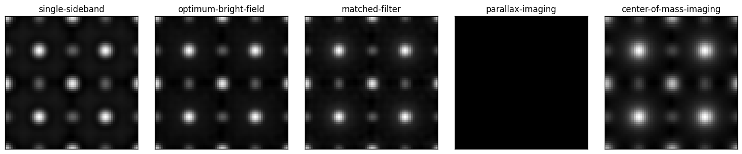
Which kernel works best depends heavily on defocus. Parallax reconstructs by shifting virtual bright-field images into alignment, and in focus there are no shifts to measure, so it returns a blank image:

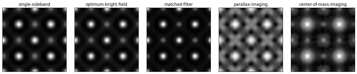
Defocus the same sample and parallax works well, showing the ring-shaped transfer pattern characteristic of defocused phase contrast:

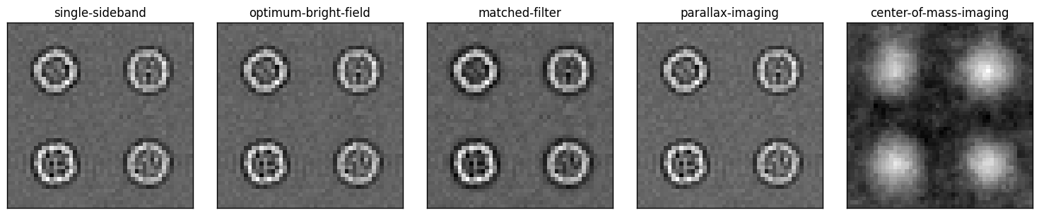
At low dose, what separates the kernels is noise and resolution. On this simulated apoferritin dataset at 100 e⁻/Ų, the four overlap-based kernels resolve the protein shell, while center of mass recovers only a blurred envelope:

Reconstructing with your chosen kernel¶

direct.reconstruct(
    deconvolution_kernel="ssb",
    upsampling_factor=2,
    q_lowpass=None,
    max_batch_size=2**8,
).visualize()

phase = direct.obj

Setting upsampling_factor above 1 reconstructs onto a grid finer than the scan step. This recovers real detail rather than interpolating, because the resolution limit comes from the aperture and not from how finely you scanned. It has no effect on 'icom'. Upsampling uses a lot of memory, so lower max_batch_size if the GPU runs out.

Measuring defocus, astigmatism, and scan rotation¶

Three quantities have to be right before any of these methods work, and none of them can be read off the microscope reliably. The defocus displayed on the instrument often disagrees with the true defocus, sometimes even in sign. The astigmatism is rarely zero. The scan rotation, meaning the angle between the scan axes and the detector axes, is a property of the microscope’s optics that has to be measured.

quantEM provides four ways to determine them. All four score candidate values by how sharply the virtual bright-field images align, and any of them can be followed by a normal reconstruction using the values it found.

Bayesian optimization is the general-purpose choice, and the one to reach for first. Search with a fast kernel, then reconstruct with a sharper one:

from quantem.diffractive_imaging.direct_ptychography import OptimizationParameter

direct = direct.optimize_hyperparameters(
    aberration_coefs={
        "C10":   OptimizationParameter(-1.5 * PROBE_DEFOCUS, -0.5 * PROBE_DEFOCUS),
        "C12":   OptimizationParameter(0, 300),
        "phi12": OptimizationParameter(-np.pi / 2, np.pi / 2),
    },
    rotation_angle=OptimizationParameter(rot - 0.2, rot + 0.2),
    n_trials=100,
    deconvolution_kernel="parallax",
)
direct.reconstruct(deconvolution_kernel="ssb", upsampling_factor=2).visualize()

Budget roughly 50 trials for each parameter you are fitting, so the example above with four parameters wants a few hundred.

Grid search tries every combination on a coarse grid. It costs more than Bayesian optimization but shows you the whole landscape rather than just the best point, which is useful when you suspect several distinct solutions. Give each parameter an n_points and call grid_search_hyperparameters.

Cross correlation measures how far the virtual bright-field images shift relative to one another, then solves for the defocus, twofold astigmatism, and rotation that would produce those shifts. Unlike the two searches above, it needs no starting guess:

direct = direct.fit_hyperparameters_cross_correlation(
    alignment_method="reference",
    bin_factors=(3, 2, 1),
)

Each entry in bin_factors is one refinement pass, binning the images by that factor before aligning them. Binning trades resolution for signal to noise, so the sequence (3, 2, 1) locks onto a rough alignment first and then refines it. On low dose data, start coarser.

Least squares fits the phase of the aperture overlap function directly. It is the only one of the four that reaches aberrations beyond defocus and twofold astigmatism:

direct = direct.fit_hyperparameters_least_squares(
    aberration_coefs={"C10": 0},
    cartesian_basis="low_order",     # C10, C12_a, C12_b, C21_a, C21_b, C30
    num_q_modes=6,
    q_signal_weight=0.5,
)

Set q_signal_weight near zero when the scan is finely sampled, and around 10 when it is undersampled.

Whichever method you use, the results are stored in direct.hyperparameter_state, which keeps your initial values and the fitted values separate. Call .summarize() to print both, and pass use_initial_state=True to reconstruct to fall back to the originals.

Passing the results to an iterative reconstruction¶

The fitted aberrations become the starting probe for iterative ptychography. For a multislice reconstruction, subtract half the total object thickness from the defocus first. Aberration fits describe the probe at the middle of the specimen, but the multislice model starts at the entrance surface:

coefs = direct.aberration_coefs.copy()
coefs["C10"] -= SLICE_THICKNESS * (NUM_SLICES - 1) / 2

Watch the units when you carry the rotation across. DirectPtychography works in radians, while preprocess on the ptychography dataset expects degrees, so convert with np.rad2deg.