With sufficient probe overlap, a single-slice ptychographic reconstruction is typically well determined, because the overlapping probe positions provide considerably more measurements than there are unknowns in the object and probe. Regularization is nonetheless useful in this regime, since it suppresses noise and discourages solutions that fit the data but are not physically sensible.
The situation changes as the model is extended. Each additional slice and each additional probe mode introduces new unknowns without providing any new measurements, and multislice or mixed-state reconstructions can therefore become underdetermined. Depth information in particular is weakly constrained. In these cases regularization is no longer merely helpful, but is required in order to obtain a meaningful solution.
quantEM provides two approaches. In the first, the object is stored on a pixel grid and explicit constraints are applied to it. In the second, the object is generated by a neural network whose architecture imposes the prior implicitly. Both approaches address the same problem, and in practice they are often combined.
Constraints on a pixelated object
Constraints are passed to reconstruct as a dict keyed by module. Any keys you omit keep their defaults.
ptycho.reconstruct(
    num_iters=50,
    constraints={
        "object": {"gaussian_sigma": 0.5, "tv_weight_xy": 10},
        "probe":  {"center_probe": True},
        "dataset": {"center_scan_positions": True},
    },
)
They fall into three groups. Hard projections are applied to the array after each update, such as clipping negative potential. Filters smooth or band-limit the object each iteration. Soft penalties are added to the loss and shape the gradient rather than the result directly.
Object constraints
| Key | Default | Effect |
|---|---|---|
positivity | True | Clips negative values in a potential object |
positivity_mode | "clamp" | "shrink" subtracts a per-slice background before clipping, which promotes atomicity |
fix_potential_baseline | False | Holds the background level of a potential object |
fix_potential_baseline_factor | 1.0 | Strength of the above; small values near 0.1 usually work best |
identical_slices | False | Forces all slices equal, for a genuinely 2D object |
apply_fov_mask | False | Restricts the object to the illuminated field of view |
gaussian_sigma | None | Gaussian blur in pixels, a smoothness prior |
q_lowpass, q_highpass | None | Butterworth band limits in Å⁻¹ |
butterworth_order | 4 | Sharpness of those band limits |
tv_weight_xy | 0 | Total variation in the image plane, edge preserving |
tv_weight_z | 0 | Total variation along the beam, for multislice |
surface_zero_weight | 0 | Pushes the outermost slices toward zero potential |
Probe and dataset constraints
| Key | Default | Effect |
|---|---|---|
orthogonalize_probe | True | Re-orthogonalizes mixed-state probe modes each iteration |
center_probe | False | Keeps the probe centered, useful when probe drift competes with position refinement |
tv_weight | 0.0 | Total variation on the probe |
center_scan_positions | False | Prevents the whole reconstruction translating during long runs with position refinement |
clip_scan_positions | True | Keeps refined positions inside the object array |
descan_tv_weight | 0.0 | Smooths fitted descan shifts across the scan |
Choosing constraints
We generally recommend applying constraints sparingly. Each constraint encodes an assumption about the specimen, and an overly aggressive constraint will suppress genuine signal along with the noise. Positivity combined with shrinkage is particularly aggressive in the early iterations of a reconstruction. For biological specimens embedded in vitreous ice, positivity is not appropriate at all, because the potential difference between protein and surrounding water can be negative.
In our experience the most valuable constraints are applied to the probe rather than to the object. Fixing the Fourier amplitude of the probe to a measured vacuum probe substantially reduces the dimensionality of the problem, and prevents object features from being absorbed into the probe, which is a common failure mode and can be difficult to detect.
Deep generative priors
A deep generative prior (DGP) replaces the pixel grid with a small convolutional neural network, using a U-Net architecture, which generates the object. The reconstruction then optimizes the weights of this network rather than the individual pixel values.
The regularization arises from the architecture of the network itself. Convolutional networks represent spatially coherent, piecewise-smooth structures readily, and represent unstructured noise only with difficulty, so noise is suppressed without any explicit penalty term. No pre-training on external datasets is required, and no ground truth is used at any stage. These networks are also referred to as deep image priors in the literature.
Relative to a pixelated object with hand-tuned constraints, deep generative priors offer several advantages:
Improved robustness to noise at low dose, with a measurably better information limit.
Faster convergence, particularly at the low spatial frequencies that pixelated reconstructions recover only slowly.
Physically plausible depth regularization in multislice reconstructions, without requiring strong explicit penalties.
Substantially less parameter tuning, since the default architecture performs well across a range of specimen types.
In the example below, a simulated test object reconstructed with a deep generative prior for 30 iterations is comparable in quality to a pixelated reconstruction requiring 250 iterations:
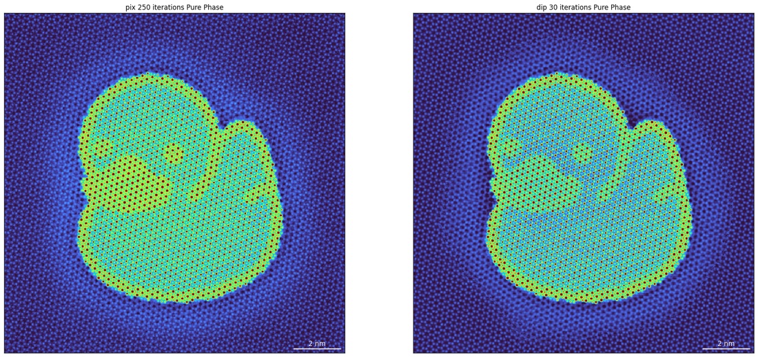
Each iteration is more expensive, often by a factor of several, but considerably fewer iterations are required, and so the total time to a converged reconstruction is typically reduced.
Running a deep prior reconstruction
PtychoLiteDIP handles the whole setup, including pretraining:
from quantem.diffractive_imaging import PtychoLite, PtychoLiteDIP

# a short pixelated run supplies the starting estimate
ptycho_pix.reconstruct(num_iters=5, reset=True, lr_obj=5e-2, lr_probe=5e-2)

ptycho_dip = PtychoLiteDIP.from_ptycholite(
    ptycholite=ptycho_pix,
    pretrain_iters=50,
    device="gpu",
)
ptycho_dip.reconstruct(
    num_iters=15,
    reset=True,
    lr_obj=5e-4,
    lr_probe=5e-4,
    scheduler_type="plateau",
).visualize()
With the full interface you build the networks yourself, which is what you want in order to control the architecture:
import torch
from quantem.core.ml import CNN2d, OptimizerParams, SchedulerParams
from quantem.diffractive_imaging import ObjectDIP, ProbeDIP

cnn_obj = CNN2d(
    in_channels=ptycho_pix.num_slices,
    start_filters=16,
    num_layers=3,
    use_skip_connections=True,
    use_batchnorm=True,
    dtype=torch.float32,             # complex64 if obj_type == "complex"
    final_activation="identity",     # "softplus" enforces positivity for potentials
)
obj_model = ObjectDIP.from_pixelated(model=cnn_obj, pixelated=ptycho_pix.obj_model,
                                     device="gpu")

cnn_probe = CNN2d(in_channels=ptycho_pix.num_probes, dtype=torch.complex64)
probe_model = ProbeDIP.from_pixelated(model=cnn_probe, pixelated=ptycho_pix.probe_model,
                                      device="gpu")

obj_model.pretrain(reset=True, num_iters=100,
                   optimizer_params=OptimizerParams.Adam(lr=1e-2),
                   scheduler_params=SchedulerParams.Plateau(factor=0.1))
probe_model.pretrain(reset=True, num_iters=100,
                     optimizer_params=OptimizerParams.Adam(lr=1e-3),
                     apply_constraints=False)
Why pre-training is required
Initializing both networks from random weights leads to unstable optimization, and such reconstructions rarely converge to a physical solution. This instability arises from simultaneously optimizing two networks through a complex forward model.
The procedure we recommend is both simple and inexpensive. First, estimate the object and probe using a conventional direct or pixelated iterative reconstruction of a few tens of iterations. Then train each network as an autoencoder, taking the corresponding estimate as input and reproducing it as output. This pre-training is fast and stable, because each network is trained independently without traversing the ptychographic forward model, and it is performed only once.
The from_pixelated constructors configure this automatically, using the pixelated model as the pre-training target.
Choosing the architecture
The depth of the network is the principal parameter to consider, and it trades convergence speed against susceptibility to overfitting.
num_layers | Behavior |
|---|---|
| 2 | Most resistant to overfitting, but cannot fully capture the low-frequency background |
| 3 | Our recommended default, which performs well across specimen types |
| 4 | Fastest low-frequency convergence, but overfits quickly and is roughly twice as expensive per iteration |
We use start_filters=16 by default, and occasionally find that a wider network helps when the probe is difficult to recover. Set final_activation="softplus" to enforce positivity for a potential object, noting that this makes the network somewhat harder to train, and "identity" otherwise.
Learning rates for deep generative priors are typically one to three orders of magnitude smaller than those used for pixelated objects, with values between 1e-4 and 5e-4 being common.
Detecting overfitting
Deep generative priors converge quickly, and beyond the optimal point they begin to reproduce noise. To identify this point, we hold out approximately 10% of the probe positions as validation data, and stop at the iteration where the validation loss reaches its minimum:
ptycho.preprocess(obj_padding_px=(32, 32), val_ratio=0.1, val_mode="random")
...
import numpy as np
best_iter = int(np.argmin(ptycho.val_iter_losses))
Storing snapshots during the reconstruction allows the result to be recovered at that iteration without rerunning it.
Multislice reconstructions with deep priors
This approach combines naturally with the multislice workflow, in three stages. We first run approximately 50 pixelated iterations to obtain the estimates used for pre-training. We then run approximately 50 deep prior iterations with identical_slices=True, which is stable and permits higher learning rates. Finally we release the identical-slices constraint and continue with light tv_weight_z and surface_zero_weight regularization. The small depth penalty additionally suppresses a checkerboard artifact along the beam direction, which originates from the upsampling layers of the convolutional network.