Multislice and mixed-state

The basic ptychographic model makes two assumptions that real experiments violate.

The first is that the whole specimen can be treated as a single thin sheet that multiplies the probe. This holds only while the specimen is thin enough that the beam does not spread appreciably as it passes through. Multislice reconstruction removes this assumption by cutting the specimen into a stack of thin slices and propagating the beam from one to the next.

The second is that the illumination is perfectly coherent, which no real electron source is. Mixed-state reconstruction removes this assumption by describing the probe as several independent modes whose intensities add together at the detector.

The two extensions are independent, and you should add them one at a time and only when the data calls for it. Each extra slice and each extra probe mode adds unknowns that the same measurements must constrain.

When you need multislice¶

The single-slice approximation breaks down at smaller thicknesses than is often appreciated. In simulations of SrTiO₃, it fails at approximately 9 nm, where strongly scattering atomic columns accumulate more than 2π of phase and are reconstructed as rings rather than as peaks.

The following observations typically indicate that additional slices are required:

Atomic columns are reconstructed as rings or doughnut shapes rather than as solid peaks, which indicates phase wrapping.
The reconstruction is sharp in one region of the field of view and blurred in another, consistent with those regions lying at different heights within the specimen.
The loss plateaus at a noticeably poorer fit than the quality of the data would suggest.

Setting up a multislice reconstruction¶

Multislice is selected by num_slices together with slice_thicknesses, in Ångström:

NUM_SLICES = 16
SLICE_THICKNESS = 1.0

obj_model = ObjectPixelated.from_uniform(
    obj_type="potential",
    num_slices=NUM_SLICES,
    slice_thicknesses=SLICE_THICKNESS,
)

Each slice must be thin enough to individually satisfy the multiplicative approximation. Typical values range from 1 Å for atomic resolution studies up to tens of Ångström for thicker specimens at lower resolution. The product num_slices × slice_thickness should span the full thickness of the specimen.

Two further adjustments are required, and both are easily overlooked.

The defocus must be shifted to the entrance surface. Aberration fits describe the probe at the middle of the specimen, whereas the multislice model begins at the entrance surface:

coefs = direct.aberration_coefs.copy()
coefs["C10"] -= SLICE_THICKNESS * (NUM_SLICES - 1) / 2

PtychoLite performs this shift automatically when middle_focus=True is set.

The object padding must be increased. The probe expands as it propagates through the slices, and if the array is too small, the expanded probe wraps around and corrupts the reconstruction. Thick objects require substantially more padding than single-slice reconstructions, frequently 64 pixels or more.

Stabilizing the depth profile¶

Depth information is weakly constrained by the measurements. An unconstrained multislice reconstruction contains many more parameters than the data supports, and the most common failure is that atoms are smeared along the beam direction rather than being confined to a single slice.

We recommend beginning with a constrained reconstruction and then relaxing it:

# Stage 1: force all slices identical, which is a stable single-slice-like solve
ptycho.reconstruct(
    num_iters=20,
    constraints={"object": {"identical_slices": True}},
    optimizer_params={"object": OptimizerParams.Adam(lr=1e-4),
                      "probe":  OptimizerParams.Adam(lr=1e0)},
)

# Stage 2: release the slices, add light depth regularization
free = ptycho.clone()
free.reconstruct(
    num_iters=50,
    constraints={"object": {
        "identical_slices": False,
        "positivity_mode": "shrink",
        "tv_weight_z": 5,
        "surface_zero_weight": 10,
    }},
)

tv_weight_z penalizes variation along the beam and speeds convergence, but too much of it smears atomic contrast in depth. surface_zero_weight pushes the potential toward zero at the top and bottom slices, which is correct whenever the specimen is embedded in vacuum.

With good data and this treatment, individual atomic layers can be cleanly separated. The depth cross-section below, taken through a reconstruction of twisted bilayer WSe₂, resolves the two layers along the beam direction:

Depth cross-section through a multislice reconstruction showing atomic columns separated along the beam direction

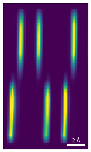
To display depth sections at the correct aspect ratio, rescale by the ratio of slice thickness to lateral sampling:

rsc_fac_z = ptycho.slice_thicknesses[0] / ptycho.sampling[0]

Inspect the slices individually with show_obj_slices(cbar=True), and take quantitative depth profiles with linescan.

Mixed-state probes¶

All real electron sources are partially coherent, both spatially and temporally. Mixed-state ptychography models this partial coherence as an incoherent sum over several mutually orthogonal probe modes, whose intensities are added at the detector.

Reconstructing partially coherent data using a single probe does not simply result in a loss of information. The mismatch in coherence is instead absorbed into the object as artifacts, and the resulting object is therefore incorrect rather than merely degraded.

probe_model = ProbePixelated.from_params(
    probe_params={"energy": PROBE_ENERGY,
                  "defocus": PROBE_DEFOCUS,
                  "semiangle_cutoff": PROBE_SEMIANGLE},
    num_probes=6,
)

The modes are re-orthogonalized at every iteration by the orthogonalize_probe constraint, which is enabled by default. Two practical observations are worth noting. Smaller batch sizes update the probe more frequently and assist the separation of the modes. Additionally, an extra mode of low intensity can usefully absorb scan-grid artifacts that would otherwise be incorporated into the object.

The number of modes required depends on both the instrument and the dose, and between four and eight is typical for atomic resolution studies of materials. We recommend starting with a single probe, and adding modes only when the reconstruction indicates that coherence is limiting, for example when probe intensity appears outside the aperture or unexplained residual structure remains. For many low dose datasets, additional modes provide no benefit, and each one substantially increases the number of free parameters.

Computational cost of these extensions¶

Both extensions are computationally expensive. The computation scales approximately linearly with the number of slices and again with the number of probe modes, while the memory requirement scales with the product of the two. As a reference point, a reconstruction using 16 slices and 4 probe modes on a 448 × 448 scan requires approximately 30 seconds per iteration on a single modern GPU. See Scaling up for the available options when this becomes limiting.