Calibration

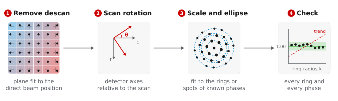
Orientation matching and strain mapping compare the detected peaks with reciprocal lattice vectors in Å⁻¹, so the peak positions must first be converted from detector pixels. We calibrate in four steps: remove the descan, measure the rotation between the detector and the scan, fit the pixel size and elliptic distortion against known phases, and check every candidate phase. All steps operate on the detected peaks rather than the diffraction images, and the result is a DiffractionCalibration that can be saved and applied to other datasets.

The examples use the titanium dataset of MacLaren et al. (2024), starting from the peaks found in Bragg disk detection.

Removing the descan¶

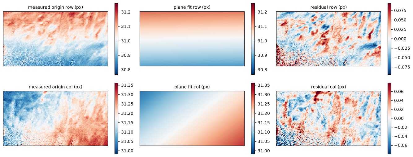
Imperfect descan moves the direct beam across the detector as the probe scans. measure_origins takes the brightest peak near the detector center as the direct beam at each position and fits a plane over the scan. correct_peak_origins subtracts the fitted origins and returns a corrected copy of the peaks:

origins = bv.measure_origins(search_radius=6.0)
bv_centered = bv.correct_peak_origins(origins, origin_ref=(0.0, 0.0))

fig, axs = bv.plot_origin_fit(origins, search_radius=6.0)

For the titanium scan, the residuals of the plane fit follow the shapes of the alpha laths, which suggests they come from the specimen rather than the descan:

If the direct beam is far from the detector center, pass its approximate position as center.

Scan rotation¶

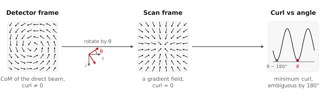
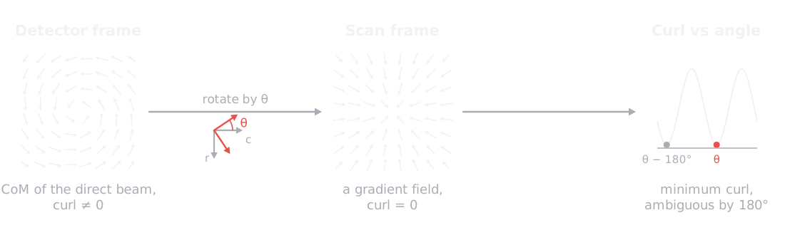
The detector axes are usually rotated relative to the scan axes. This rotation sets the in-plane orientations and strain directions, while zone axes and phases do not depend on it. measure_scan_rotation finds it from the center of mass of the direct beam, which in the scan frame is the gradient of the projected potential and therefore has no curl. Rotating the detector axes until the curl vanishes gives the angle, up to 180°, and a transposed detector is tested as well:

rotation = bv.measure_scan_rotation(origins, plot=True)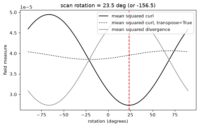

The result is written to the dataset metadata, where calibrate, calibrate_2d, strain mapping, and ptychography read it. In crystalline specimens, diffraction contrast can dominate the center of mass. For the titanium scan the curl changes by less than a factor of two with angle, and measure_scan_rotation warns that its result of 23.5° is unreliable. We therefore use the 34° reported by MacLaren et al. (2024), passed as rotation_ccw_deg below. A rotation measured by ptychography in the same session can be used the same way.

Pixel size and elliptic distortion¶

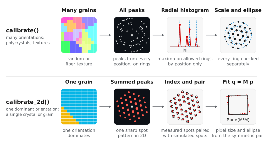
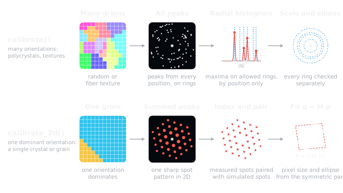
Two routines fit the pixel size and elliptic distortion. Choose by the texture of the specimen:

Both take the candidate phases as Crystal objects with structure factors calculated:

from ase.build import bulk
from quantem.diffraction import Crystal

ti_alpha = Crystal.from_ase(
    bulk("Ti", "hcp", a=2.9505, c=4.6855),
    name="Ti alpha",
).calculate_structure_factors(k_max=1.5)

ti_beta = Crystal.from_ase(
    bulk("Ti", "bcc", a=3.26, cubic=True),
    name="Ti beta",
).calculate_structure_factors(k_max=1.5)

Rings: calibrate¶

calibrate matches the measured ring radii to the rings the reference crystals allow, using positions only. Every allowed ring counts equally and a missing ring costs nothing, so texture and dynamical intensities do not bias the scale. The scale is scanned within ±10% of the guess, the ellipse and scale are refined in turn, and each ring is then checked separately:

cal = bv_centered.calibrate(
    [ti_alpha, ti_beta],
    pixel_size_guess=0.038,     # 1/Angstrom per pixel
    rotation_ccw_deg=34.0,
    plot=True,
)
print(cal)

DiffractionCalibration(pixel_size=0.038422 1/A/px, ellipse: e11 +0.00586 e12 +0.00605, rotation 34 deg, 12 rings, rms 0.18%)

The figure compares the measured peaks with the alpha rings before (left) and after (right) the fit, as a radial histogram (top) and as azimuth against scattering vector (bottom):

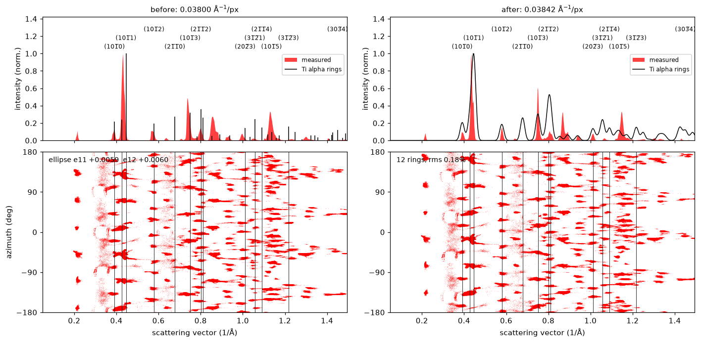
Ring radii repeat at fixed ratios, so a position-only match is unique only over a limited range of scales. Keep the guess within about 10%, and widen scale_search only for a guess that is far out. calibrate warns when the fit is unreliable, including when the peaks cover too few azimuths to fix the ellipse, which indicates that calibrate_2d is the better choice.

Spots: calibrate_2d¶

When one orientation dominates the scan, the summed peaks form a single sharp spot pattern. calibrate_2d indexes this pattern against the candidate crystals, pairs the measured and simulated spots, and fits a 2 × 2 map from pixels to Å⁻¹. The symmetric part of the map gives the pixel size and ellipse, and the rotation part belongs to the crystal orientation:

cal = bv_centered.calibrate_2d(
    [ti_alpha, ti_beta],
    pixel_size_guess=0.038,
    energy_ev=200e3,
    precession_deg=0.5,
    rotation_ccw_deg=34.0,
    plot=True,
)
print(cal)

DiffractionCalibration(pixel_size=0.038418 1/A/px, ellipse: e11 +0.00385 e12 +0.00483, rotation 34 deg, Ti beta, 27 spots, rms 0.0025 1/A)

The beta matrix of the titanium alloy is a single grain, so its spots dominate the summed pattern. The figure shows the beta rings (top) and the 2D histogram of every peak in red under the simulated spots in black (bottom), before and after the fit:

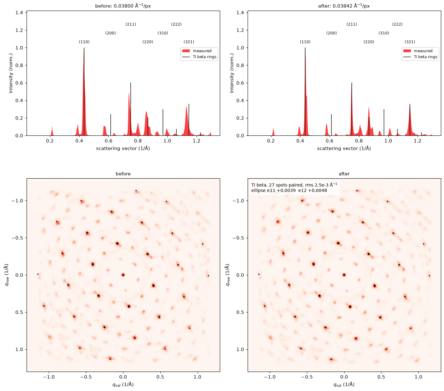
calibrate_2d needs a guess within a few percent, which calibrate can provide. Within one zone axis, a lattice parameter error of the reference cannot be distinguished from detector ellipticity, so the reference should be a well-known structure. For this scan the two routines agree to 0.01%.

Subsets of positions¶

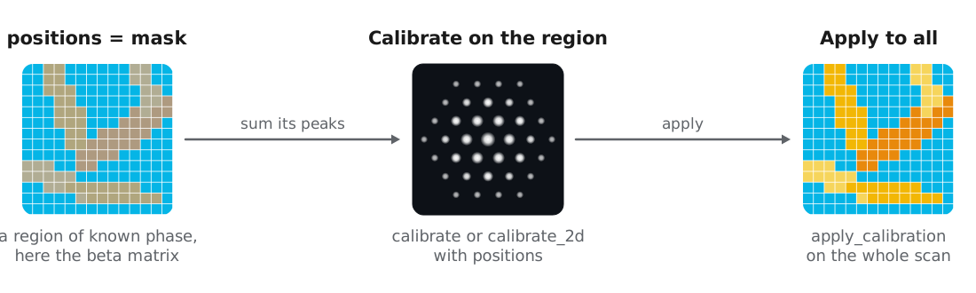
Both routines accept positions, a list of (row, col) or an (R, C) boolean mask, to calibrate on a region whose crystallography is known, such as one grain or a standard particle in the field of view. The calibration is then applied to the whole scan. Here we use masks of each phase from a previous phase map:

# mask_alpha, mask_beta: (R, C) boolean masks, e.g. cm.mask("Ti beta") > 0.5
cal_beta = bv_centered.calibrate_2d(
    ti_beta, 0.038, energy_ev=200e3, precession_deg=0.5, positions=mask_beta,
)
cal_alpha = bv_centered.calibrate(ti_alpha, 0.038, positions=mask_alpha)

The beta matrix alone gives 0.038425 Å⁻¹/px and the alpha laths alone give 0.038431 Å⁻¹/px, within 0.04% of the values from the whole scan.

Applying and reusing a calibration¶

A DiffractionCalibration stores the pixel size, ellipse, rotation, and transpose, together with the evidence behind them: the matched rings or spots and their residuals. apply_calibration converts the centered peaks to Å⁻¹, and the returned Vector carries the calibration with it:

peaks = bv_centered.apply_calibration(cal)

Calibrating against the specimen assumes its lattice parameters are known. For strained specimens, or phases whose lattice parameters vary with composition, we recommend calibrating on a standard such as nanocrystalline gold, saving the result, and applying it to the specimen. rebin converts a saved calibration to data with a different detector binning:

gold = Crystal.from_ase(
    bulk("Au", "fcc", a=4.078, cubic=True),
    name="Au",
).calculate_structure_factors(k_max=1.5)

# bv_au_centered: detected and centered peaks of the gold standard
cal_au = bv_au_centered.calibrate(gold, pixel_size_guess=0.038)
cal_au.save("calibration_Au.zip")

from quantem.core.io.serialize import load

peaks = bv_centered.apply_calibration(load("calibration_Au.zip"))

Checking every phase¶

A phase with the wrong lattice parameter can still give a good overall fit, and matching cannot recover from it, so we check each candidate phase before matching. plot_ring_comparison shows the radial histogram of the calibrated peaks against the rings of each crystal:

from quantem.diffraction import CrystalMap

cm = CrystalMap.from_vectors(peaks, [ti_alpha, ti_beta], energy_ev=200e3, precession_deg=0.5)
fig, axs = cm.plot_ring_comparison()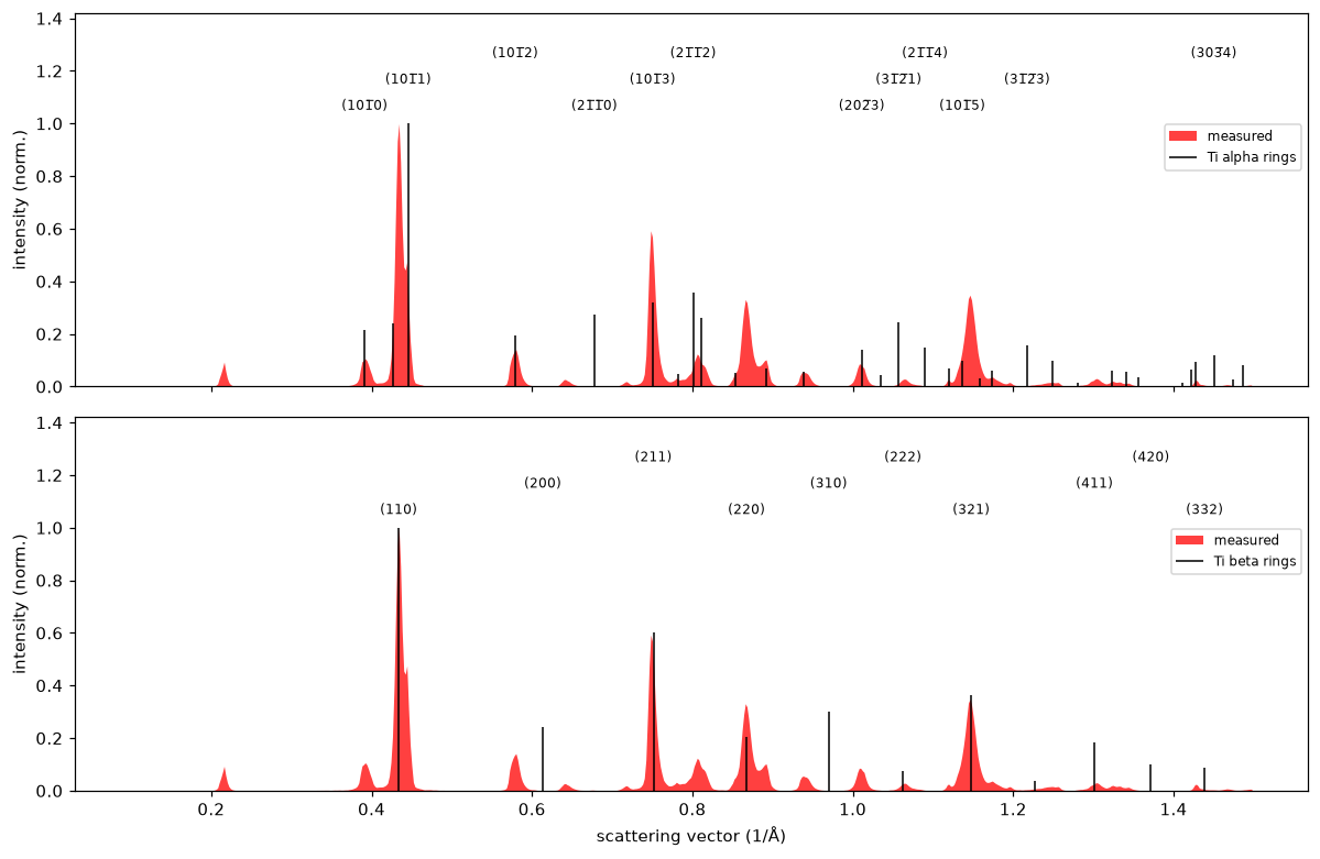

Both phases line up with the measured peaks. The strongest alpha and beta rings nearly overlap, a consequence of the orientation relationship between the phases described in orientation and phase mapping. plot_calibration adds the azimuth of every peak, where a ring that wobbles with azimuth indicates remaining elliptic distortion, and plot_bragg_rings draws the rings over the Bragg vector map in 2D:

fig, ax = cm.plot_bragg_rings(n_rings=6)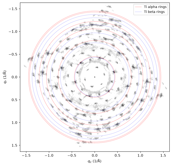

Refining the calibration from strain¶

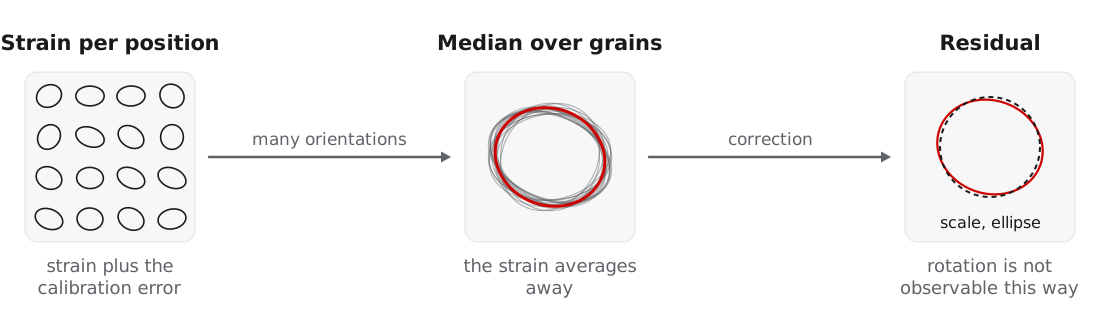
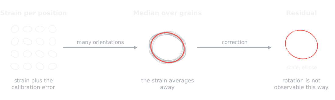
After orientation mapping, the deformation fitted at each position by calculate_strain contains both the local strain and any global calibration error. refine_calibration takes the median deformation over many differently oriented grains, which averages the strain away and leaves the residual scale and ellipse:

from quantem.diffraction import calibration

strain_maps = [cm[name].calculate_strain(mask=cm.mask(name) > 0.5) for name in cm.names]
residual = calibration.refine_calibration(strain_maps)
peaks = calibration.transform_peaks(peaks, residual["correction"])

For the titanium scan, the median over 17,715 positions gives a residual scale of 0.05% and a residual ellipticity below 0.1%, which confirms the calibration from calibrate_2d.

The detector rotation is absorbed into the fitted orientations and cannot be refined this way.

Lower-level functions¶

The routines above are built from functions in quantem.diffraction.calibration, which can be used directly: