Orientation and phase mapping

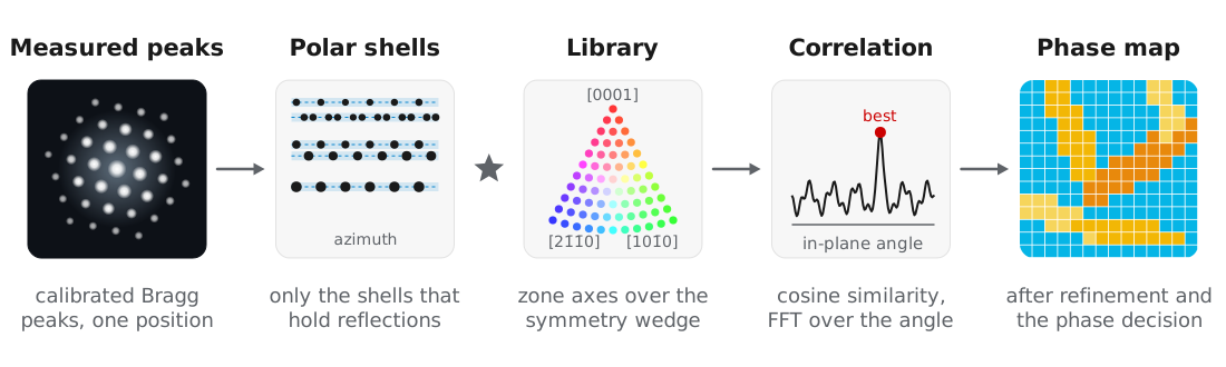
Automated crystal orientation mapping (ACOM) determines the orientation and phase at every probe position by matching each measured pattern to a library of simulated patterns. Rauch et al. (2010) demonstrated this approach using precession electron diffraction, where rocking the beam over a cone (Vincent and Midgley, 1994) makes the measured intensities closer to kinematical simulations.

quantEM uses the sparse correlation matching introduced in py4DSTEM by Ophus et al. (2022), which represents the library and the measured peaks in polar coordinates and evaluates the correlation only on radial shells that contain reflections. The library match is followed by refinement of each orientation, a phase decision between the candidate crystals, and a measurement of projected strain. All of these steps use the calibrated peaks from Bragg disk detection and Calibration.

Example dataset¶

The examples use the scanning precession electron diffraction dataset of an alpha-beta titanium alloy from MacLaren, Frutos-Myro, Zeltmann, and Ophus (2024): hcp alpha laths in a bcc beta matrix, recorded at 200 kV with 0.5° precession over 100 × 191 probe positions. We thank Ian MacLaren (University of Glasgow) for sharing the data, and ask that you cite MacLaren et al. (2024) if you use it. The binned file is Ti550_005_downsampled.h5.

Candidate structures¶

Each candidate phase is a Crystal, built from ASE or from a CIF file with Crystal.from_cif. Crystal finds the symmetry with spglib and restricts the library to the fundamental zone axis wedge, since symmetry-related orientations give identical patterns:

from ase.build import bulk
from quantem.diffraction import Crystal

ti_alpha = Crystal.from_ase(
    bulk("Ti", "hcp", a=2.9505, c=4.6855),
    name="Ti alpha",
    pseudo_symmetry_tol=0.01,
).calculate_structure_factors(k_max=1.5)

ti_beta = Crystal.from_ase(
    bulk("Ti", "bcc", a=3.26, cubic=True),
    name="Ti beta",
    pseudo_symmetry_tol=0.01,
).calculate_structure_factors(k_max=1.5)

Ti alpha
  space group      P6₃/mmc (194)
  point group      6/mmm   (Laue class 6/mmm)
  pseudo-symmetry  none found at tol = 0.01 (0.030 A)
  matching         12 proper rotations, zone axis wedge [0001], [101̅0], [21̅1̅0]
Ti beta
  space group      Im-3m (229)
  point group      m-3m   (Laue class m-3m)
  pseudo-symmetry  none found at tol = 0.01 (0.033 A)
  matching         24 proper rotations, zone axis wedge [001], [011], [111]

pseudo_symmetry_tol lets a structure that is close to a higher symmetry be matched with that symmetry, so that orientations no experiment can tell apart are not sampled separately.

Building the orientation library¶

A CrystalMap holds one orientation map per candidate crystal and carries the phase decision. build_plan simulates the library of each crystal:

from quantem.diffraction import CrystalMap

cm = CrystalMap.from_vectors(
    peaks,                      # calibrated peaks
    [ti_alpha, ti_beta],
    energy_ev=200e3,
    precession_deg=0.5,
)
cm.build_plan(
    angle_step_zone_axis_deg=1.0,
    angle_step_in_plane_deg=5.0,
    corr_kernel_size=0.05,
    sigma_excitation=0.02,
    power_intensity=0.25,
    device="mps",               # or "cuda", or "cpu"
)

Ti alpha: orientation plan 1862 zone axes x 72 in-plane angles, 32 radial shells, matching 6/mmm
Ti beta: orientation plan 1127 zone axes x 72 in-plane angles, 11 radial shells, matching m-3m

Each library pattern is a kinematical simulation averaged over the precession cone, described in Diffraction simulation. The in-plane angle can be sampled coarsely because the correlation over it is computed by FFT and refined afterwards.

Testing the match on a few positions¶

Matching the full scan takes several minutes, so we first check a few positions:

test_positions = [(50, 130), (26, 76), (30, 121), (80, 40)]

phase_colors = ["#E36C0A", "#1155CC"]   # alpha, beta

cm.match_orientations(positions=test_positions, num_matches=2, min_number_peaks=4)
fig, axs = cm.plot_matches(
    positions=test_positions, matches=(0,), transpose_plots=True, colors=phase_colors,
)

The best alpha (orange, top row) and beta (blue, bottom row) candidates are drawn over the measured peaks (gray):

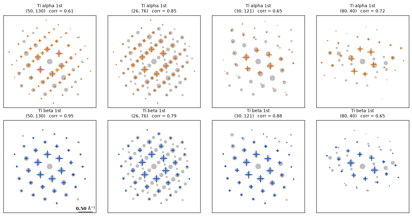
The correlation is a cosine similarity between 0 and 1. It saturates on sparse patterns, where a direct beam and two noise peaks can score as well as a real grain, so we use it only to rank orientations of one crystal. With num_matches=2, the second match is fit to the peaks the first leaves unexplained, so a probe straddling two grains indexes both.

Running the full scan¶

cm.match_orientations(num_matches=2, min_number_peaks=4)
cm.refine_orientations(num_iterations=5, zone_search_deg=1.5)
cm.fit()

print({k: round(v, 3) for k, v in cm.phase_fractions().items()})

{'unindexed': 0.005, 'Ti alpha': 0.487, 'Ti beta': 0.507}

The full scan takes about 5 minutes on a laptop.

Refinement. refine_orientations removes the quantization of the library. The in-plane rotation is fit by least squares to the paired peak positions, and the zone axis tilt is fit to the measured intensities, since peak positions in the zero-order Laue zone carry almost no tilt information. Positions that disagree with their neighbors are then retried with the neighbors’ orientations as candidates.

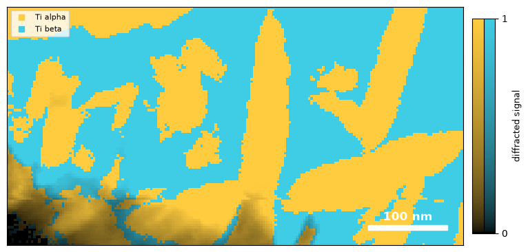
Phase decision. fit tests how well each candidate pattern, and each pair of patterns, explains the measured peaks, and assigns the phase of the lowest-cost model. Positions with almost no diffracted peaks, such as vacuum or amorphous regions, are left unindexed.

fig, ax = cm.plot_phase()

Color gives the phase and brightness the diffracted signal:

The correlation maps show why the phase decision does not compare correlations directly:

fig, axs = cm.plot_correlation(mask=True)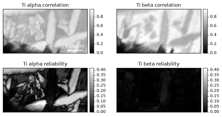

The beta correlation is high over most of the scan, including the alpha laths, because the strong reflections of the two phases nearly coincide. The reliability, the margin between the best orientation and the next distinct one, is near zero for beta everywhere: the matrix indexes as two orientations rotated 60° about ⟨111⟩, which give nearly identical patterns. Reliability therefore measures how well an orientation is determined, and does not test whether the crystal is present.

Orientation maps¶

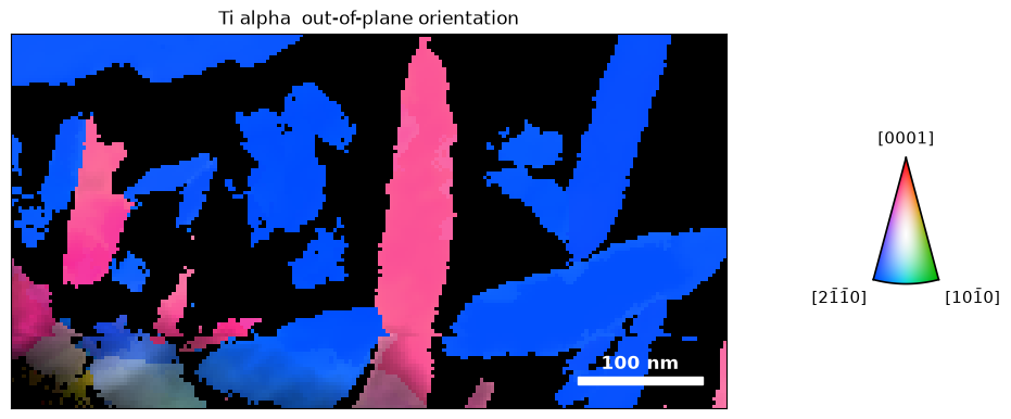
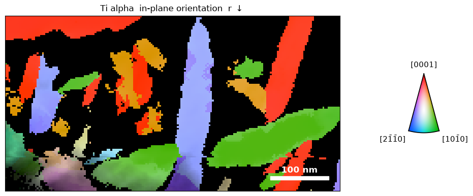
plot_orientation draws inverse pole figure maps of each phase, masked by the phase decision. The smooth option averages neighboring orientations for display only:

figs = cm.plot_orientation(
    smooth=dict(sigma_px=1.0, sigma_deg=1.0, max_angle_deg=5.0),
)

The out-of-plane map colors each position by the crystal direction along the beam. Most alpha laths are viewed close to ⟨21̄1̄0⟩ (blue):

The in-plane map colors by the direction along the scan rows, and separates laths that share an out-of-plane orientation:

Orientation relationship¶

Pole figures show the orientation relationship between the phases. We plot the alpha (0001) poles and overlay the beta ⟨110⟩ poles:

fig, ax = cm.plot_pole_figure(
    pole=(0, 0, 1),
    phase="Ti alpha",
    color_by="ipf",
    label="(0001)",
    overlay={
        "om": cm["Ti beta"],
        "pole": (1, 1, 0),
        "mask": cm.mask("Ti beta"),
        "label": "<110> beta",
    },
)

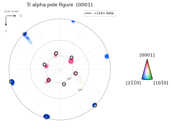
The alpha basal poles fall on the beta ⟨110⟩ poles, as expected for the Burgers orientation relationship, (0001)α ∥ {110}β (Burgers, 1934). Alpha poles that miss the overlaid circles belong to the second beta variant.

Projected strain¶

calculate_strain fits the 2 × 2 in-plane deformation that maps the refined simulated peaks onto the measured peaks at each position. The reference is the ideal lattice of each phase, so no strain-free region is needed:

strain_alpha = cm["Ti alpha"].calculate_strain(
    mask=cm.mask("Ti alpha") > 0.5,
    ds_sampling=30.0,
    ds_units="A",
)
fig, ax = strain_alpha.plot_strain(
    rotation_angle=0.0,                 # strain axes along the scan rows and columns
    strain_range_percent=(-2.0, 2.0),
)

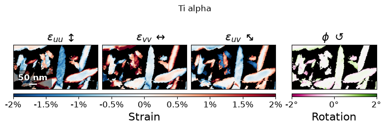
Errors in the pixel size or the assumed lattice parameters appear as a uniform strain over a whole phase, so variations in strain are more reliable than its mean value. refine_calibration uses this to estimate the remaining calibration error from many grains (see Calibration). The measurement is averaged through the specimen thickness.

Inspecting individual fits¶

example_positions selects the clearest examples of each phase, or with ambiguous=True, the closest decisions:

positions = cm.example_positions(ambiguous=True, num=3)
fig, axs = cm.plot_matches(positions=positions, dataset=dataset, matches=(0,), colors=phase_colors)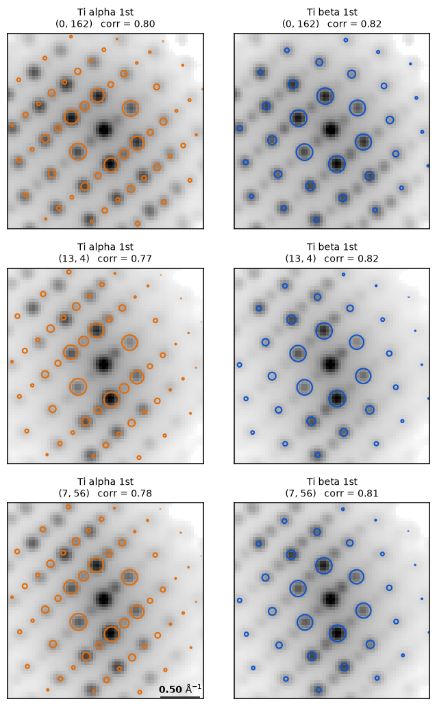

In these patterns, the strong reflections of both phases coincide, and the decision rests on weaker reflections that only one phase predicts.

Saving the analysis¶

cm.save("Ti_crystal_map.zip", mode="o")

The saved CrystalMap can be refined further with CrystalMap.refine_dynamical, which fits Bloch wave intensities to determine orientation, thickness, and phase at each position (see Diffraction simulation).