Bragg disk detection

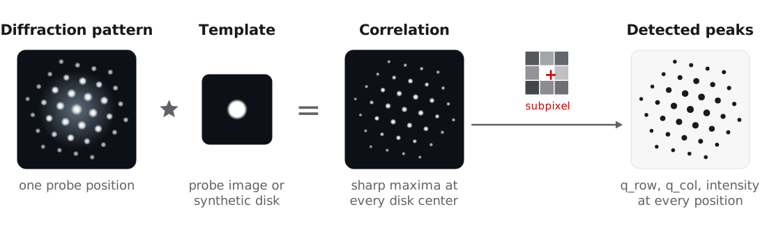
In nanobeam and 4D-STEM experiments, each Bragg reflection appears as a disk on the detector, and the disk centers give the projected reciprocal lattice at each probe position. BraggVectors finds these disks by template matching: each pattern is cross-correlated with an image of one disk, and the maxima of the correlation are refined to subpixel positions. The detected peaks are the input to calibration, orientation and phase mapping, and strain mapping.

This approach follows the template matching in py4DSTEM (Savitzky et al., 2021). Pekin et al. (2017) compared cross, phase, and hybrid correlation for disk registration, and all three are available through the corr_power parameter. The examples use the titanium dataset of MacLaren et al. (2024), described in orientation and phase mapping.

Building a template¶

No vacuum probe was recorded for the titanium dataset, so we use a synthetic disk matched to the direct beam:

from quantem.core.io.file_readers import read_emdfile_to_4dstem
from quantem.diffraction import BraggVectors

dataset = read_emdfile_to_4dstem("Ti550_005_downsampled.h5")
dataset.sampling = [30.0, 30.0, 1.0, 1.0]       # 30 Angstrom scan step
dataset.units = ["A", "A", "pixels", "pixels"]

bv = BraggVectors.from_dataset(dataset)
bv.make_template_synthetic(radius=0.75, edge=1.0)

Detection parameters¶

detect_params = dict(
    min_abs_intensity=40.0,
    min_spacing=4.0,
    edge_boundary=2.0,
    background_sigma=1.0,
    subpixel="upsample",
    upsample_factor=16,
    max_num_peaks=500,
)

Testing on a few positions¶

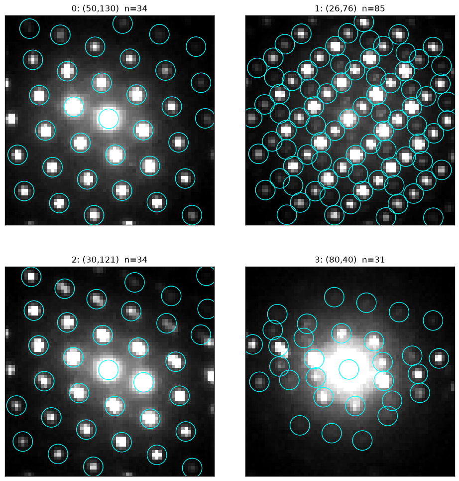
We recommend tuning these parameters on a few probe positions before running the full scan. show_detection draws the detected peaks without changing the workflow state:

test_positions = [(50, 130), (26, 76), (30, 121), (80, 40)]

bv.show_detection(
    positions=test_positions,
    **detect_params,
    peak_radius=3,
    ncols=2,
    norm={"power": 1.0, "upper_quantile": 0.95},
)

Detecting the full scan¶

peaks_px = bv.detect_disks(**detect_params)

The 19,100 patterns of the titanium scan take about 10 s on a laptop CPU, and batching makes detection faster still on a GPU (BraggVectors.from_dataset(dataset, device="cuda")). The peaks are stored in bv.peaks as a Vector of [q_row, q_col, intensity] in detector pixels. They still include the descan and have no reciprocal space calibration, which the next step, calibration, corrects.